The double pendulum in Maxima
José A Vallejo
Faculty of Sciences
State University of San Luis Potosí (México)
URL: http://galia.fc.uaslp.mx/~jvallejo
Email: jvallejo@fc.uaslp.mx
ABSTRACT: This wxMaxima worksheet is just an adaptation of the really amazing Physics Lab
presented in https://www.myphysicslab.com/pendulum/double-pendulum-en.html (which is
done in Javascript). Go there for details of the dynamics and to see a wonderful interactive
applet.
1 Theoretical preliminaries
First, we consider the equations resulting from the balance of forces. For the upper pendulum
we have:
| (%i1) | eq1:m[1]·a[x,1]=−T[1]·sin(%theta[1])+T[2]·sin(%theta[2]); |
| (%i2) | eq2:m[1]·a[y,1]=T[1]·cos(%theta[1])−T[2]·cos(%theta[2])−m[1]·g; |
For the lower pendulum:
| (%i3) | eq3:m[2]·a[x,2]=−T[2]·sin(%theta[2]); |
| (%i4) | eq4:m[2]·a[y,2]=T[2]·cos(%theta[2])−m[2]·g; |
In https://www.myphysicslab.com/pendulum/double-pendulum-en.html, the first step to
get the equations of motion is
| (%i5) | eq5:eq1+eq3; |
| (%i6) | eq6:eq2+eq4; |
The second step consists in
| (%i7) | eq7:cos(%theta[1])·eq5; |
| (%i8) | eq8:sin(%theta[1])·eq6; |
From these, we get (in the third step):
| (%i9) | eq7+eq8; |
or
| (%i10) | eq9:ratsimp(%); |
Now we do something similar with the lower pendulum, but just in one shot:
| (%i11) | cos(%theta[2])·eq3+sin(%theta[2])·eq4; |
| (%i12) | eq10:ratsimp(%); |
In https://www.myphysicslab.com/pendulum/double-pendulum-en.html it is stated that
these are equations for %alpha[1], %alpha[2], the second derivatives of %theta[1], %theta[2],
respectively. This is so because we have some orther relations (in which we are using
the notation %omega[1], %omega[2] for the first derivatives of %theta[1], %theta[2] with
respect to time):
| (%i13) | a[x,1]:−(%omega[1])^2·L1·sin(%theta[1])+%alpha[1]·L1·cos(%theta[1]); |
| (%i14) | a[y,1]:(%omega[1])^2·L1·cos(%theta[1])+%alpha[1]·L1·sin(%theta[1]); |
| (%i15) | a[x,2]:a[x,1]−(%omega[2])^2·L2·sin(%theta[2])+%alpha[2]·L2·cos(%theta[2]); |
| (%i16) | a[y,2]:a[y,1]+(%omega[2])^2·L2·cos(%theta[2])+%alpha[2]·L2·sin(%theta[2]); |
Taking this into account, equations eq9 and eq10 become (notice the use of '' to evaluate
a[i,j])
| (%i17) | eq11:''eq9; |
| (%i18) | eq12:''eq10; |
Now, we want to solve for the angular accelerations %alpha[1] and %alpha[2]. This is easy for
Maxima (or any other CAS), because the equations are linear with respect to those variables:
| (%i19) | solve([eq11,eq12],[%alpha[1],%alpha[2]]); |
Let us reorganize the output in a more manageable form:
| (%i20) | ratsimp(trigreduce(%)); |
These are exactly the final equations of motion presented in https://www.myphysicslab.com/pendulum/double-pendulum-en.html
2 The numerical solution
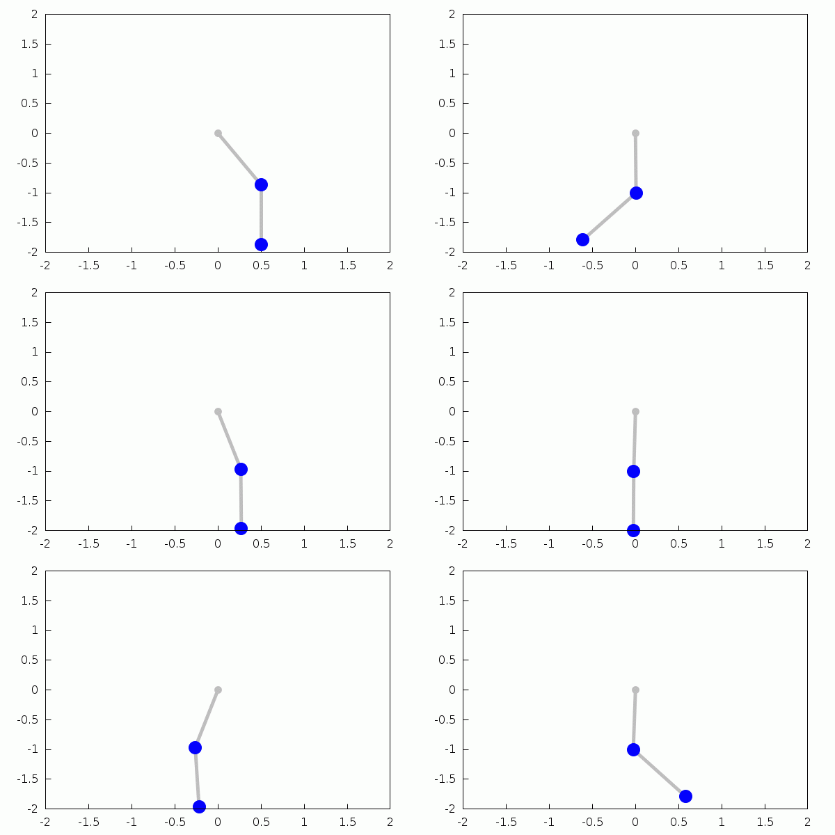
We will use the Runge-Kutta method. Here is a Maxima function that directly generates the
animation. Notice how we transform from the variables (%theta[1],%theta[2],%omega[1],%omega[2])
to (x1,y1,x2,y2) (and we only use (x,y) to actually represent the double pendulum):
| (%i21) |
double_pendulum(L1,L2,m1,m2,g,t10,t20,w10,w20,tspan,tstep,ff):=block( [%theta1,%theta2,%omega1,%omega2,expr1,expr2,expr3,expr4,tmp,N,soln1,soln2,wxanimate_framerate:ff], expr1:%omega1, expr2:%omega2, expr3:−((m2·sin(2·%theta2−%theta1)+(−m2−2·m1)·sin(%theta1))·g+2·m2·%omega2^2·sin(%theta2−%theta1)·L2+%omega1^2·m2·sin(2·%theta2−2·%theta1)·L1)/ ((m2·cos(2·%theta2−2·%theta1)−m2−2·m1)·L1), expr4:(((m2+m1)·sin(%theta2−2·%theta1)+(m2+m1)·sin(%theta2))·g+m2·%omega2^2·sin(2·%theta2−2·%theta1)·L2+(2·%omega1^2·m2+2·m1·%omega1^2)·sin(%theta2−%theta1)·L1)/ ((m2·cos(2·%theta2−2·%theta1)−m2−2·m1)·L2), tmp:rk([expr1,expr2,expr3,expr4],[%theta1,%theta2,%omega1,%omega2],[t10,t20,w10,w20],[t,0,tspan,tstep]), N:length(tmp), soln1:makelist([L1·sin(k[2]),−L1·cos(k[2])],k,tmp), soln2:soln1+makelist([L2·sin(k[3]),−L2·cos(k[3])],k,tmp), with_slider_draw(l,makelist(m,m,1,N), xrange=[−L1−L2,L1+L2], yrange=[−L1−L2,L1+L2], point_type=filled_circle, color=gray, points([[0,0]]), points_joined=true, line_type=solid, line_width=5, points([[0,0],soln1[l]]), points([soln1[l],soln2[l]]), color=blue, point_size=3, points_joined=false, points([soln1[l],soln2[l]]) ) )$ |
The syntax is more or less clear, but here are the details (in all cases, the subscript 1 refers
to the upper pendulum and 2 to the lower pendulum):
L1, L2 lengths of the rods,
m1, m2 masses of the bobs,
g value of gravitational constant,
t10, t20 initial values of the angular displacements (short for %theta1[0] and %theta2[0]),
w10, w20 initial values of the angular velocities,
tspan is the total time the animation will run,
tstep is the tiem step in the Runge-Kutta method (some value around 0.05 is enough),
ff is the animation framerate.
Here is an example:
| (%i22) | double_pendulum(1,1,2,2,9.8,%pi/6,0,0,0,5.5,0.05,17); |
 \[\tag{%o22} \]