the initial value x[0] for 0
| (%i16) | wxevolution(F(0.8,x),0.9,10); |
Dynamical systems with Maxima
1 The continuous case
The most basic model for population growth is given by the equation
dP(t)/dt=k·P(t) (1)
where P(t) is the population at time t and k is a constant, positive
if P(t) is increasing, or negative if P(t) is decreasing.
However, this model is not very accurate in the long run. It does not
take into account those factors that put a limit on P(t) or dP(t)/dt,
such as the availability of nutrients, or the spreading of diseases
when P(t) is a big number.
A simple modification of (1) which considers these possibilities is
achieved with the introduction of a parameter k=k(P), depending on the
population in such a way that it decreases when P increases.
The simplest case is
k=a-b·P, a,b>0 (2)
so (1) reads now
dP(t)/dt=P(t)·(a-b·P(t)). (3)
When P(t)~0, equation (3) basically reduces to (1) with k~a, but for
higher values of P(t), the product b·P approaches a, so dP/dt~0 and
the growth slows down.
With the changes of variables
P=a·x/b, dP/dt=(a/b)·dx/dt (4)
equation (3) becomes (making now k=a)
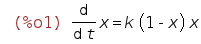
dx/dt=k·x·(1-x) (5)
which is called the logistic equation (it was introduced by P. F.
Verhulst in 1838 and popularized in its discrete version by R. May in
1976).
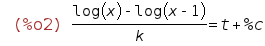
The equation (5) is separable, and so readily solved:
| (%i1) | 'diff(x,t)=k*x*(1-x); |
| (%i2) | ode2(%,x,t); |
| (%i3) | method; |
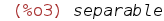
Note that the variable "method" stores the procedure followed by Maxima
to solve the equation. Let us set the initial conditions x(t=0)=x0:
| (%i4) | ic1(%o2,t=0,x=x[0]); |
We can try to make the solution explicit:
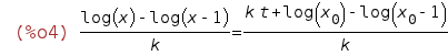
| (%i5) | logcontract(%); |
We can see here the limitations of Maxima when simplifying...
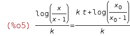
Anyway, the equation is very simple and we can help Maxima a little
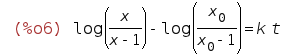
by writing
| (%i6) | log(x/(x-1))-log(x[0]/(x[0]-1))=k*t; |
Then, everything goes fine:
| (%i7) | logcontract(%); |
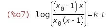
| (%i8) | solve(%,x); |
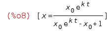
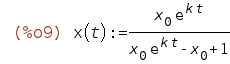
Thus, we have our explicit solution in the form
| (%i9) | x(t):=(x[0]*%e^(k*t))/(x[0]*%e^(k*t)-x[0]+1); |
Let us plot it, to see the asymptotic behaviour. We take the values
k=1.5 and x[0]=0.1:
| (%i10) | wxplot2d(subst([k=1.5,x[0]=0.1],x(t)),[t,0,10]); |
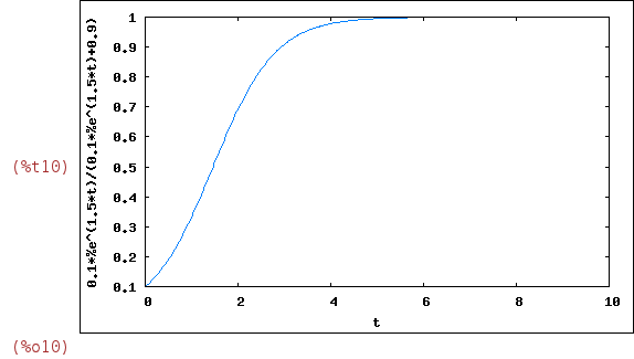
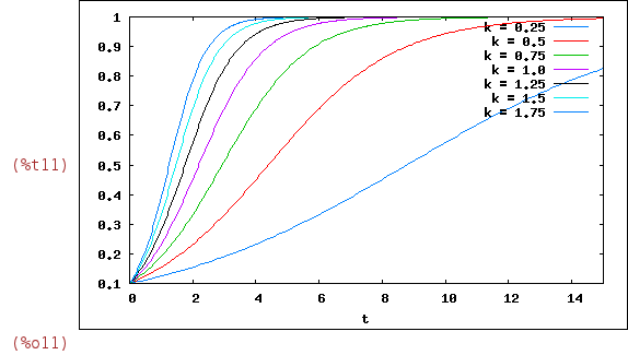
Note that, due to the normalization (4), all the solutions x(t)~1 for
large values of t. The parameter k influences the slope of the curve, as
we can see by plotting together several of them, for different values of
k (in the example, ranging from k=0.25 to k=1.75 with increments of 0.25)
| (%i11) |
wxplot2d( makelist(subst([k=d*(0.25),x[0]=0.1],x(t)),d,1,7), [t,0,15], cons(legend,makelist(k=d*(0.25),d,17)) ); |
2 The discrete case
The discrete version of equation (5) is called the logistic map, and
is given by the difference equation
x[n+1]=r·x[n]·(1-x[n]) (6)
where we will assume r>0.
A fundamental feature of this equation, absent in the continuous case,
is that (6) can not be explicitly solved. We must use qualitative or
numerical methods to obtain information about the solutions. For instance,
letting f[n](x)=r·x[n]·(1-x[n]) (the second memeber of (6)), we note that
those values x=c for which f[n](c)=c are the only constant (or equilibrium)
solutions x[n]=c. They are easily computed in Maxima:
| (%i12) | solve(r*c*(1-c)=c,c); |
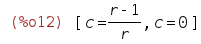
Considering our knowledge of the behaviour of the solutions to a 1D (continuous)
differential equation, we would expect that the solutions would evolve around
these constant solutions x[n]=0 and x[n]=(r-1)/r or escape to infinity. But,
surprisingly, this does not happen!.
Let us graphically see the behaviour for several values of r. First we define,
once for all, our model:
| (%i13) | F(r,x):=r*x*(1-x); |

Then, we make use of the following command wxevolution, which computes the
n+1 points given by x[i+1]=F(x[i]) when i runs from 0 to n, starting from
an initial value x[0] (in this example, we take x[0]=0.1), and plot the result
within the wxMaxima session (this is a small modification of the built-in
evolution command). We begin with r=0.25:
| (%i14) |
wxevolution(fun, initial, n, [options]) := block ([z:initial, data: [[0, initial]], kwds: [], plot: numer: true, float: true], if length(listofvars(fun)) # 1 then error("fun should depend on one variable"), for i thru n do (z: ev(fun, listofvars(fun)[1]=z), if not numberp(z) then error("The function gave a non-numerical value:", z), data: cons([i, z], data)), for i thru length(options) do (if not listp(options[i]) then error("Wrong option", options[i]), kwds: cons(options[i][1], kwds)), if not member('x,kwds) then options: cons(['x, -0.5, n+0.5],options), if not member('xlabel,kwds) then options: endcons(['xlabel, "n"],options), if not member('ylabel,kwds) then options: endcons(['ylabel,concat(listofvars(fun)[1],"(n)")],options), if not member('style,kwds) then options: endcons(['style,'points],options), options: cons(['discrete, data], options), apply(wxplot2d, options))$ |
| (%i15) | wxevolution(F(0.25,x),0.1,10); |
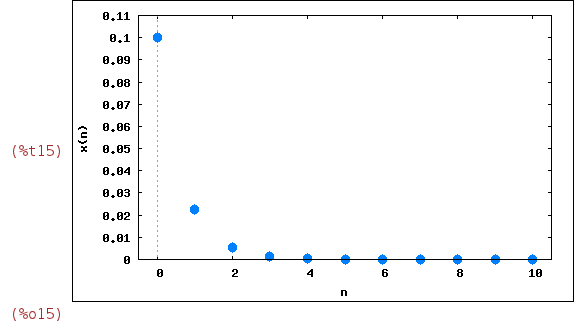
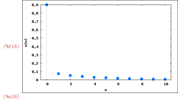
Thus, we see that the population dies. Indeed, it ends this way independently of
the initial value x[0] for 0
(%i16)
wxevolution(F(0.8,x),0.9,10);
A little experimentation shows that the behaviour follows the guidelines:
▷ When 1 > r > 0, the population will eventually die, independent of the initial population.
▷ When 2 > r > 1, the population will quickly approach the value (r-1)/r, independently of the initial population.
▷ When 3 > r > 2, the population will also eventually approach the same value (r-1)/r, but first will fluctuate
around that value for some time. The rate of convergence is linear, except for r=3, when it is less than linear.
▷ When 1+√6 > r > 3 (1+√6 ~ 3.45), from almost all initial conditions the population will approach
permanent oscillations between two values. These two values are dependent on r.
▷ When 3.54 > r > 3.45 (approximately), from almost all initial conditions the population will approach permanent oscillations among four values.
▷ With r increasing beyond 3.54, from almost all initial conditions the population will approach oscillations among 8 values,
then 16, 32, etc. The lengths of the parameter intervals which yield oscillations of a given length decrease
rapidly; the ratio between the lengths of two successive such bifurcation intervals approaches the so-called Feigenbaum
constant, F=4.669.... This behavior is called a "period-doubling cascade".
Let us check some examples. We choose the intial condition x[0]=0.5:
| (%i17) | wxevolution(F(1.3,x),0.5,10); |
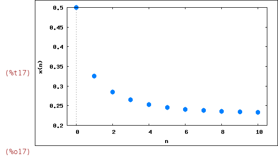
Note that (1.3-1)/1.3 ~ 0.23. Now we take r=2.4, x[0]=0.55:
| (%i18) | wxevolution(F(2.4,x),0.55,15); |
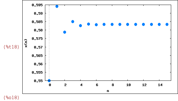
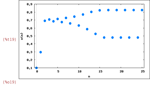
We begin observing interesting things by choosing r=3.3 and x[0]=0.1:
| (%i19) | wxevolution(F(3.3,x),0.1,25); |
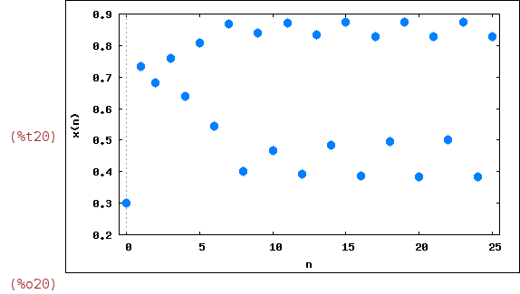
And here we take r=3.5, x[0]=0.3:
| (%i20) | wxevolution(F(3.5,x),0.3,25); |
3 Staircase diagrams
We have seen the appearance of "double" and "quadruple" points of equilibrium
in the last two examples. There is another graphical method to study these
points, which we now describe. It is based on the fact that the dynamics is
given by
x[n+1]=F(r,x[n])
where F(r,x) was defined in %i13: in the case of the logistic map, F(r,x):=r·x·(1-x).
Thus, in a plane where its points (x,y) represent the population values in two
consecutive steps, (x,y)=(x[n],x[n+1]), this point is the intersection of the vertical
line x=x[n] and the parabola y=F(r,x[n]). Once x[n+1] is known, to obtain the next
value x[n+2] we force x[n+1] to play the role of x[n] in the previous step. So we
carry x[n+1] to the horizontal axis by taking the intersection of the horizontal line
y=x[n+1] with the bisectrix y=x. Then, x[n+2]=F(r,x[n+1]) and the whole process is
iterated again and again. In this way, we get the orbit of the system starting from
any initial condition x[0].
Maxima has a command staircase to generate these graphics; we modify it in order
to display the graphics inside the wxMaxima session, the resulting command is called
wxstaircase. Let us see an example:
| (%i21) |
wxstaircase(fun, initial, n, [options]) := block ([zf, z:initial, z1:initial, z2:initial, stair:[[initial, initial]], kwds: [], numer: true, float: true], if length(listofvars(fun)) # 1 then error("fun should depend on one variable"), for i thru n do (zf: ev(fun, listofvars(fun)[1]=z), if not numberp(zf) then error("The function gave a non-numerical value:", zf), stair: append(stair, [[z, zf], [zf, zf]]), z: zf, if z < z1 then z1: z, if z > z2 then z2: z), for i thru length(options) do (if not listp(options[i]) then error("Wrong option", options[i]), kwds: cons(options[i][1], kwds)), if not member(listofvars(fun)[1],kwds) then options: cons([listofvars(fun)[1], 4*(1.1*z1-.1*z2)/3,4*(1.1*z2-.1*z1)/3],options), if not member('y,kwds) then options: endcons(['y,1.1*z1-.1*z2,1.1*z2-.1*z1],options), if not member('xlabel,kwds) then options: endcons(['xlabel,concat(listofvars(fun)[1],"(n)")],options), if not member('ylabel,kwds) then options: endcons(['ylabel,concat(listofvars(fun)[1],"(n+1)")],options), if not member('legend,kwds) then options: endcons(['legend,false],options), options: cons([['discrete, stair], fun, listofvars(fun)[1]], options), apply(wxplot2d, options))$ |
| (%i22) | wxstaircase(3.3*x*(1-x),0.1,25,[x,0,1]); |
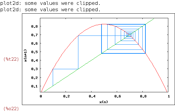
Here we see that the orbits go from one point of equilibrium (x~0.48) to another
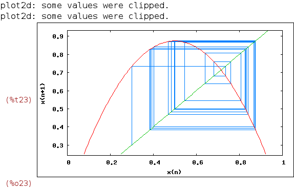
(x~0.85),as in %o19. We can also reproduce the behaviour of %o20, where there are
four equilibrium points (we iterate 75 times to see better the density of the orbits
around the equilibrium points. Note that each "square" intersected with the diagonal
defines two points):
| (%i23) | wxstaircase(3.5*x*(1-x),0.3,75,[x,0,1]); |
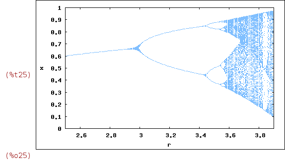
4 Bifurcations
We have seen that the behaviour of the solutions of the logistic map depends on
the value of the parameter r. Indeed, starting with r~3.45 the number of equilibrium
points start to vary, in a kind of "doubling cascade". We can study the change in
the structure of the solutions as r varies, through the use of bifurcation diagrams.
In these, we plot in the horizontal axis the different values of the parameter r.
For each of them, we compute the number of fixed points which are "attractors" for
the orbits, and represent this number in the vertical axis (only the "stable" values
are considered, although we will not discuss the meaning of this condition).
Maxima can do that with its built-in command orbits, which we modify in order to
display the graphic inside our wxMaxima session:
| (%i24) |
wxorbits(f, y0, n1, n2, domain, [options]) := block ([x, y, data: [], y1, y2, yflag: false, kwds: [], var, points, plot: [], x0: domain[2], s, n, pixels: 600, numer:true, float: true], var: listofvars(f), var: delete(domain[1],var), if length(listofvars(fun)) >2 then error("f should depend on two variables."), for i thru length(options) do (if not listp(options[i]) then error("Wrong option", options[i]), if options[i][1]=var[1] then (y1: options[i][2], y2: options[i][3], if not y1 < y2 then error("The first number has to be smaller than the second in:",options[i]), options[i][1]: 'y, yflag: true), if options[i][1]='nticks then (if integerp(options[i][2]) then n: options[i][2] else error("Option nticks should have an integer value")), if options[i][1]='pixels then (pixels: options[i][2], delete(options[i],options)) else plot: endcons(options[i], plot), kwds: cons(options[i][1], kwds)), if not (member('nticks,kwds) and integerp(n)) then n: 200, s: (domain[3] - domain[2])/n, if yflag then (for i:0 thru n do (x: x0+i*s, y: y0, points: [], for j thru n1 do (y: ev(f, domain[1]=x, var[1]=y), if not numberp(y) then error("The function gave a non-numerical value:", y)), for j thru n2 do (y: ev(f, domain[1]=x, var[1]=y), if ((y >= y1) and (y <= y2)) then (k: entier(pixels*(y-y1)/(y2-y1))+1, if k>pixels then k: pixels, if not member(k, points) then points: cons(k, points))), for j thru length(points) do data: cons([x,(y2-y1)*(points[j]-0.5)/pixels+y1], data))) else (for i:0 thru n do (x: x0+i*s, y: y0, for j thru (n1+n2)/2 do (y: ev(f, domain[1]=x, var[1]=y), if not numberp(y) then error("The function gave a non-numerical value:", y), if not yflag then (y1:y, y2:y, yflag: true) else (if y if not y1 < y2 then error("It was not possible to find any points"), for i:0 thru n do (x: x0+i*s, y: y0, points: [], for j thru n1 do y: ev(f, domain[1]=x, var[1]=y), for j thru n2 do (y: ev(f, domain[1]=x, var[1]=y), if ((y >= y1) and (y <= y2)) then (k: entier(pixels*(y-y1)/(y2-y1))+1, if k>pixels then k: pixels, if not member(k, points) then points: cons(k, points))), for j thru length(points) do data: cons([x,(y2-y1)*(points[j]-0.5)/pixels+y1], data))), if (length(data) > 0) then (if not member('x,kwds) then (if domain[3] > domain[2] then plot: cons(['x,domain[2],domain[3]],plot) else plot: cons(['x,domain[3],domain[2]],plot)), if not member('xlabel,kwds) then plot: endcons(['xlabel,domain[1]],plot), if not member('ylabel,kwds) then plot: endcons(['ylabel,var[1]],plot), if not member('style,kwds) then plot:endcons(['style,'points],plot), plot: cons(['discrete, data], plot), apply(wxplot2d, plot)))$ |
Note that, in the next command, we restrict the plot to the iterations between n=50 and
n=200, and the initial condition is fixed at x[0]=0.1:
| (%i25) | wxorbits(r*x*(1-x), 0.1, 50, 200, [r, 2.5, 3.9], [style, dots]); |
5 Exercises
The techniques that we have explained, can be applied to any dynamical system of
the form dx/dt=F(x,t) or x[n+1]=F(r,x[n]). The reader should look for some other
examples in the literature and study them. For instance, x[n+1]=k+x[n]², or
x[n+1]=cos(k·x[n]), etc.